North America: Historical First Person Journal Observations Google Map and Datasets:
Brief Explanation and Outline
Google Earth Map updated April 4, 2024; Excel Database file (below) updated April 4, 2024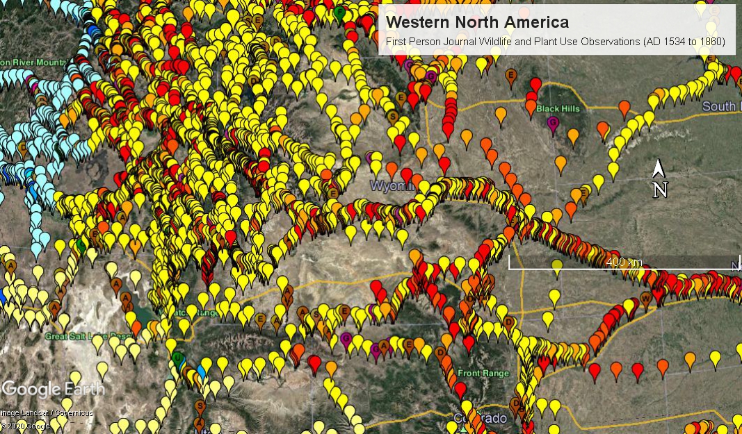

As one way to help interpret changes in vegetation visible in historic photographs, researchers can use first person journal accounts to estimate historical human, wildlife, fish and fowl densities and human use, culturing and burning of plants. The data currently start in along the eastern seaboard as Verrazzano approached the coast on March 7, 1524,  for the Southwest in November, 1528 when De Vaca and several dozen Spaniards landed on the coast of Texas, and in the Northwest on July 14, 1691 as Henry Kelsey started south across the Canadian prairies from the Saskatchewan River. For the contiguous United States the data conclude on June 30, 1860 when Captain William Raynolds descended the Madison River to Three Forks after a month long journey from the North Platte River through the Rocky Mountains, or in 1871 for the Colorado River canyonlands as Major Powell’s expedition mapped the intricacies of this complex landscape. For Canada, early traveler journals for the Arctic are tabulated into the early 1900s. In all, the data includes nearly 30,000 journal-days of locations, and wildlife and other ecological observations from such notables as De Soto, Coronado, Cartier, Champlain, Hudson, Samuel Hearne, Escalante, Alexander Mackenzie, Lewis and Clark, Peter Skene Ogden, David Thompson, David Douglas, Jediah Smith, Fremont, and Joseph Burr Tyrrell.  The main historical journal observation Excel database methodology generally follows: Kay, C.E. 2007. “Were Native People Keystone Predators? A Continuous-Time Analysis of Wildlife Observations Made by Lewis and Clark”. Canadian Field-Naturalist 121 (2007): 1-16.

Google Earth file- If you have Google Earth loaded on your computer, these should map by simply downloading the “kmz” file. On many computers, when you click on download button above, a Google Map version shows up first, with the actual “file download” toggle on the right top of the map. Click this to get the kmz file (currently about 2400KB). Yes, these Google Earth folks can sure store data efficiently. Once you have downloaded the file into your “Temporary Places”, its best to turn off all the observations, then expand the journal subfiles for NW, SW or East, and at a broad regional level click on individual traveler’s journals to get a general orientation on routes. Its best to turn off all or most the database files to move around large landscapes rapidly. Then, zoom into areas of interest and make all the journals visible for finer-scale spatial pattern analysis.  

Once you are considering individual Google Earth journal observations, basic information on each point (journalist/date) is available by right clicking on the point, and looking at “Properties”. Alternately, you can expand the legend on the left of the Google Earth map, and choose journals, periods of time, or even individual journal days. For example, by clicking on and off the visible files for trips, you have many options to look at certain trips, or periods of time. When exiting the file, you can save it in “My Places” for further viewing. 

As per the legend file on Google Earth, our “working” color coding for the Google Earth Map journal-day points is something like this:

1) Bison country: Yellow is no bison observed or no wildlife observation for day, Orange is moderate numbers, Red is many bison observed/killed.

2) Salmon country (or other fisheries): Light blue is no fishing observed, or no observation for day, grading to dark blue for major fishing observed, or occurs during some times of year (weirs, huts etc. observed).

3) Moose and caribou country: light grey is no wildlife observed, or no observation for day, grading to dark brown (with a C) for abundant caribou (edge of the barren grounds). A medium brown with a “C” indicates small group sightings (potentially mountain or woodland ecotypes). 

4) Great Basin, Colorado Plateau, southern deserts: (outside of 1800s bison range): Light yellow for “no observation” journal days.

5) California central valley and eastern United States/Canada: Light green for “no observation” days. 

6) Browns indicate abundant elk-E, deer-D, moose-M, A-antelope, G-goats, F-fowl etc. observed for day. This color coding not consistent, and as with with wildlife observations details is better interpreted through the individual species columns of the Excel files (see below).

7) Plant use: Greens including maize (M), squash (S), beans (B), quamish (camas, Q), pinyon nuts (P), acorns in CA or agave in Texas (A), general garden (G) or for construction materials (C).

8) Purple “G”s or purple Ps- Grizzly or polar bear observations. 

9) Red “C”s, “H”s, “S”s- in the southwest these are significant observations of domestic or feral cattle, horses, or sheep. Cattle and oxen were brought north as early as the 1540s by Spanish entradas into the Rio Grande and Colorado river watersheds. This adds complexity to evaluating bovid sign (e.g., tracks, bones, and hides) in this area.  

Of course, once you have opened the properties for each point you can re-color or code your points by whatever scheme meets your working needs. Or better yet, move the Excel file (see below) into a Geographic Information System and do some serious analysis.

The project has likely plotted about 90% of bison country historical journals observations currently available in the literature for the northwest area, and we are in the process of entering the observations of traveler’s journals into salmon, moose, and caribou country, and have entered substantial data for the southwest (CO, OK, NM, UT, AR, CA, NV), and northern Mexico. Substantial data has also been entered for the eastern United States and southeastern Canada.  

Excel data file– The more detailed historical  journal observations are in an Excel database linked to the spatial data points by observer-day. A key for this is at the top of the file spreadsheets (following Kay 2007, see above). The database also provides the references for the journals used to compile the data. The NW and SW main spread sheets have lat-long columns filled (unfreeze panes to see left-most columns), but the NW, SW and East  “journals in progress” may not have this data extracted from Google Earth yet.

Data Use Example 1: Northwest Bison Movement Corridors– One application of this data is to evaluate the pattern of bison movement corridors from the Great Plains into the Rocky Mountains from the Peace River south to the Platte River. This is especially interesting north and south of the Yellowstone Plateau. The repeat photograph posting for Henry’s Lake provides more detail for thinking about the South or Bozeman pass corridors. These are the “mothers of all corridors” for bison going west into the Cordillera. A brief  view of the wildlife journal data suggests a major bison dispersal event westwards over South or Bozeman passes in about 1815. The results of these investigations is also given in a detailed progress report available for downloading here. 

Data Use Example 2: Southwest Hide Trade Networks– Two great southwest eco-cultural mysteries are the collapse of the Chaco Canyon culture at about AD 1150, and the  expansion of bison onto the southern plains of Texas after about AD 1300. Perhaps these phenomena are linked, and the historical record of  human use of wildlife and plant resources, when combined with archaeological and traditional knowledge, can help untangle this relationship. A progress report on the results of this investigation are described here for downloading.   

Data Use Example 3: Factors Effecting Historical Distribution and Restoration of Bison bison- CW is working with ecologist Jonathan Farr to do multivariate analyses of potential causal patterns for the historic distribution of bison, and how these may influence current restoration projects. Our work for the northwest area is now available in the journal “Diversity”: https://www.mdpi.com/1424-2818/14/11/937/htm

Data Use Example 4: Biomes to Anthromes in the American Northwest- For over 10,000 years three  main eco-cultural biomes have evolved adjacent to each other in northwest North America: 1) coastal/plateau salmon, 2)subarctic/arctic caribou and moose, and 3) prairie and mixedwood bison. Databases of fire frequency studies and historical journal accounts compiled at the ecoregion scale can be used to evaluate whether indigenous peoples, through hunting, gathering, and culturing, were the keystone species that structured the food webs of eco-cultural biomes. Recent global-scale human population and technological growth are causing a rapid transition of these long-term biomes to “anthromes”, a set of globally-standard land use types of various levels of urbanization, agriculture, and forestry. These altered human ecosystem management practices are resulting in major changes in fire regimes and species abundance. A technical report on this research is available here for downloading.    

Suggested Reference

CW (and helpful associates) intend to keep this ongoing work and data in the public domain, so please pass along to those interested. Many types of more quantitative analyses are possible.

White, Clifford A. 2024. NA-JOBS: North America- Historical Journal Observations Google Earth Map and Database . CW and Associates, Canmore Alberta. April 4, 2024 update. Database  accessible at: https://lensoftimenorthwest.com/themes/lens-northwest-files/google-earth-map-journal-wildlife-observations/   

After c. 2026, back-up digital databases will be filed with various global biodiversity data centers,  and will be given an archival home at the Whyte Museum Archives, Banff, Alberta: https://www.whyte.org/digitalvault/categories/archives-library